Expert Commentary

At a Glance
- To determine which drivers have the greatest influence on an outcome variable, many analysts turn to techniques such as multiple linear regression, random forest, or Shapley values.
- But these methods don’t work well when several drivers are highly collinear.
- To understand overall variable importance, simple methods such as Pearson correlation can more effectively assess the strength of the relationship between a driver and the outcome variable independently of other potential drivers.
- With that understanding, managers can then address how to improve performance along the relevant drivers, either singly or in logical clusters.
Analytical techniques to perform driver analysis come in handy when a company seeks to understand a particular outcome, such as customer satisfaction or profit per store, as a function of several potential drivers. Ranking potential drivers by how strongly they affect the outcome metric allows the company to focus resources on improving performance along the right ones.
Common techniques include multiple linear regression (MLR), random forest, Shapley values, Johnson’s relative weights, partial correlations, and Pearson correlation. Many of these methods control for effects of other drivers and might not be suitable for ranking them in terms of importance. The reason they may not be suitable is the distinction (which we will explain) between concepts of overall variable importance and marginal variable importance.
Elements of Value® in retail banking
Consider the case of a retail bank trying to understand what drives customer advocacy. Data comes from a survey of 2,500 consumers, asking how likely they are to recommend a certain brand to a friend or colleague—the core Net Promoter ScoreSM question. This likelihood to recommend becomes the outcome variable, with our goal being to understand which variables have the strongest associations with this metric.
Potential drivers are a set of 30 attitudinal statements capturing how well a certain brand performs on the Elements of Value as experienced by customers (see Figure 1). The survey asked respondents to rate their experience with the bank on each Element of Value using a scale of 0–10. Delivering on multiple Elements of Value can lift products or services above commodity status.

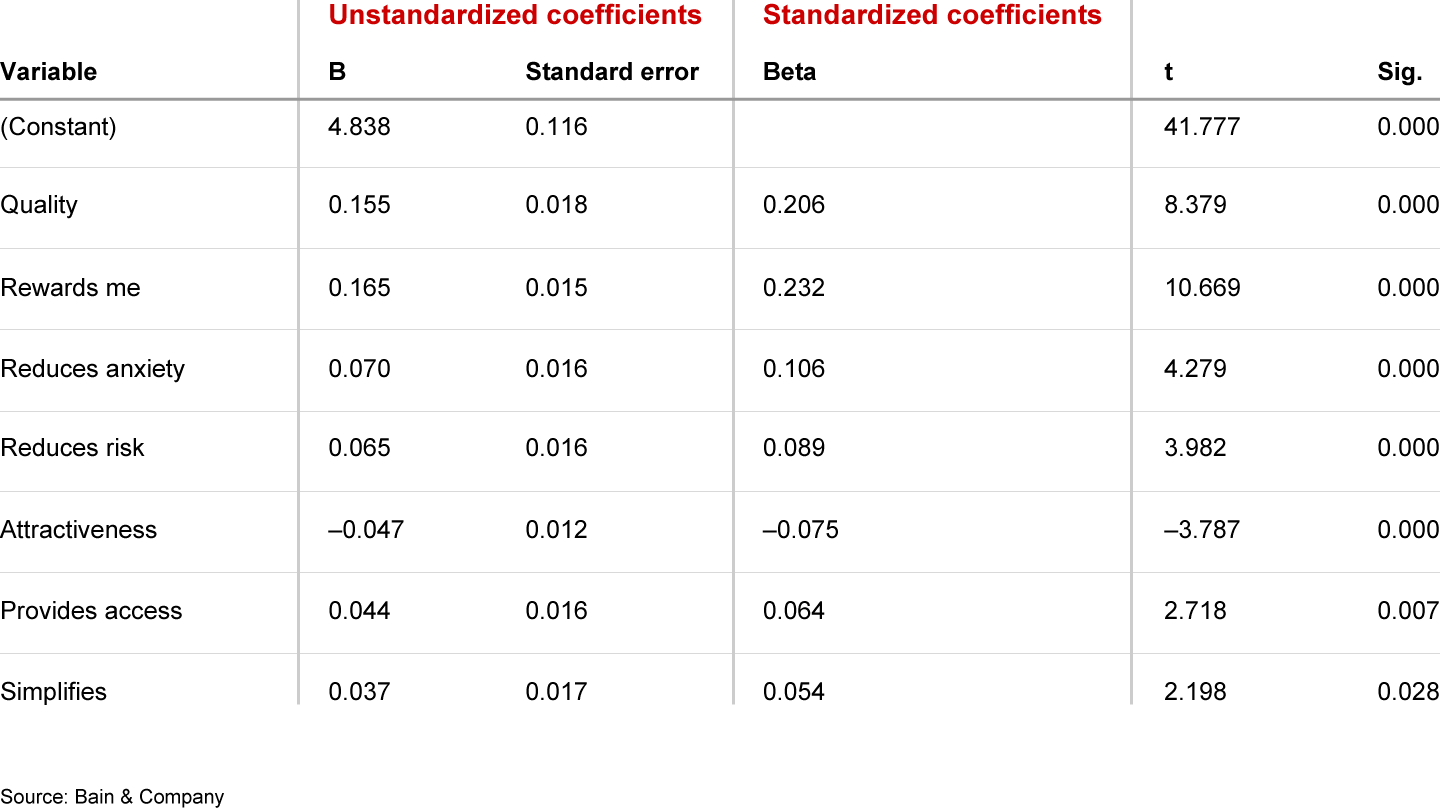
In such a scenario, some analysts would turn to MLR, interpreting standardized coefficients1 as indicators of variable importance. (Standardized coefficients imply normalization of driver variables for differences in scale, so standardized coefficients are more comparable across variables than raw coefficients.) Anyone familiar with MLR knows that for a model to produce meaningful results, one must first select the appropriate variables. As is common in psychometric research, some of the 30 drivers correlate highly with others, a phenomenon called multicollinearity. Figure 2 contains model coefficients as well as additional statistical metrics for each driver selected by the algorithm.

Here we need to acknowledge that a set of variables included in MLR will differ depending on how the analyst selects them. A hypothesis-driven approach ensures the highest possible interpretability of the model. But regardless of the approach, the analyst can only include a subset of variables in the model. After we removed insignificant variables, 7 of our 30 potential ones remained. The other 23 were excluded because they lacked relevance for predicting the outcome variable, or because of high collinearity with drivers already included in the model.
Because collinearity was one reason for excluding certain variables, we cannot conclude that the seven drivers included in the model are the only important ones. In other words, MLR didn’t produce a ranking of all potential drivers by their importance.
As for the seven included in the model, can we interpret coefficients as being relative levels of importance of each driver included in the model? Coefficients of MLR indicate what increase in the outcome variable is associated with a one-unit increase in each driver, keeping other drivers constant. In this case, though, it’s not possible to keep those constant. When drivers are collinear, which often happens with psychometric statements, improving one will likely improve others as well. MLR coefficients thus have limited practical importance here.
MLR can still prove useful for predicting how the outcome variable would change if the company improved drivers included in the model.
How random forest falls short
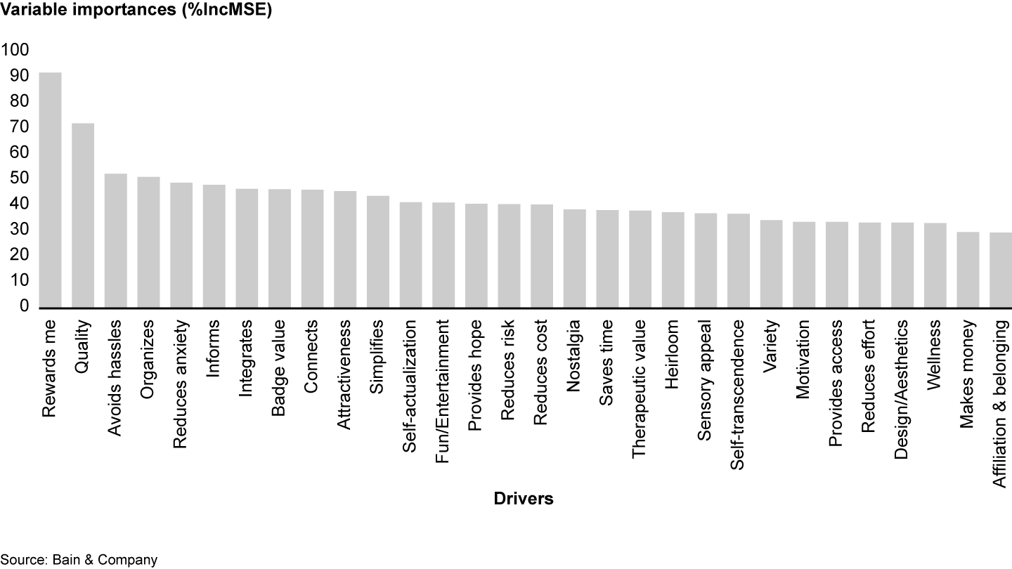
Turning to another common predictive method, random forest,2 a useful feature of this algorithm is that it estimates how model performance would suffer if you left out a particular variable. (Random forest is an ensemble method that constructs a large number of decision trees and produces a mean or mode prediction depending on whether the dependent variable is numerical or categorical. We used the programming language R’s randomForest package and kept the default value of mtry hyperparameter—that is, the number of drivers divided by 3, or in our case mtry=10. Ntree=5,000.) We rank our drivers from highest to lowest according to random forest’s metric of variable importance, %IncMSE3 (see Figure 3). IncMSE is defined as a percentage increase in Mean Squared Error after a driver was randomly permuted. It indicates a decrease in accuracy associated with leaving a certain driver out of the model.

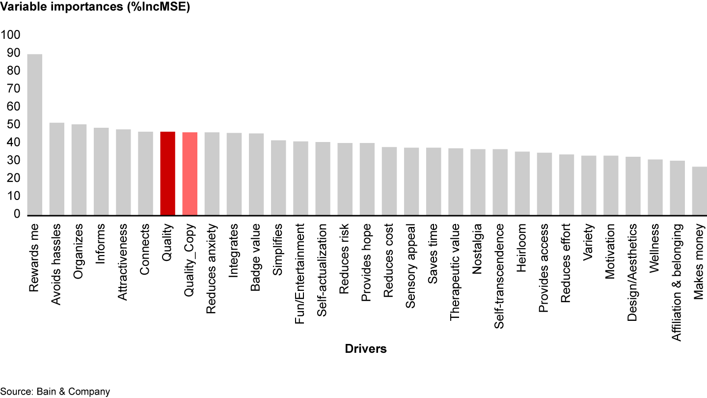
As discussed earlier, psychometric data typically features high collinearity between some of the drivers. When choosing a method for analyzing variable importance, we need to make sure it provides robust results even when drivers are highly collinear. An important driver should, in theory, still be important even if it is collinear with others. To test whether random forest produces a reliable ranking of drivers even in cases of high degrees of collinearity, we created a duplicate of the driver ranked second, quality, and included this duplicate variable in the model. (A duplicate variable is a copy of the original variable and is the extreme case of collinearity—the correlation coefficient between the variable and the duplicate is 1.)
We would expect that duplicating a driver would have no effect on its ranking. However, in this experiment, neither “quality” nor its copy ranks second any longer (see Figure 4). Just like the MLR coefficients, the drivers in random forest were penalized for high collinearity with other drivers. (One can minimize the effect of collinearity in random forest by setting mtry=1. Such hyperparameter settings will make random forest consider only one independent variable at each split, making the decision trees less similar to each other. When using random forest for predictive purposes, though, this technique might decrease performance of the model.)

This result makes sense once we recall how random forest defines variable importance: It indicates how model performance would suffer if we left out a particular driver—an illustration of marginal variable importance. What we want to understand, though, is how strongly each driver relates to our outcome variable independent of the effect of other drivers—the phenomenon of overall variable importance.
Other methods commonly employed for driver analysis include Shapley values, Johnson’s relative weights, and partial correlations. Similar to MLR coefficients and random forest variable importance measures, scores provided by these methods are affected by the collinearity of drivers. Such collinear drivers often receive lower scores than drivers of similar predictive strength that don’t correlate with other drivers.
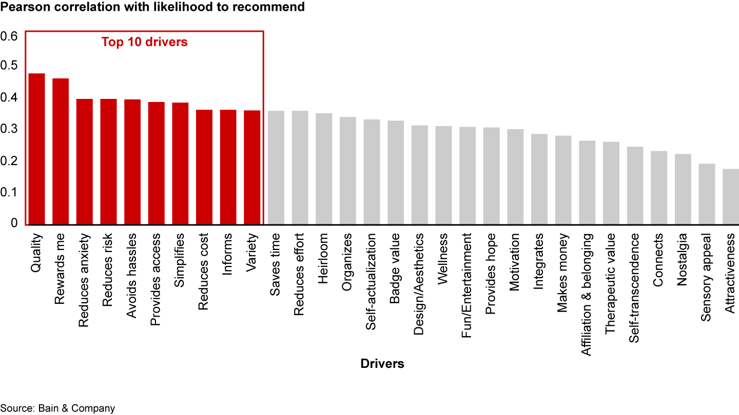
To truly understand overall variable importance, we need to explore methods that assess the strength of the relationship between a driver and the outcome variable independently of other potential drivers. The simplest, most common of such methods is Pearson correlation.
First we rank potential drivers by their importance for predicting the likelihood to recommend (see Figure 5). Note that Pearson correlations do not give reliable estimates of strength of relationships between variables if the variables are non-normally distributed, the data contains outliers, or the associations between variables are non-linear. In such cases, one should use other methods, such as Spearman rank correlation, which is more robust in the presence of outliers.

Many companies conclude their driver analysis by shortlisting the top 5 or 10 drivers. We recommend taking an additional step, namely analyzing whether top drivers are interrelated and may be addressed simultaneously. We will explore this topic in an upcoming article.
Elements of Value® is a registered trademark of Bain & Company, Inc.


